

In part 1, we looked at capacity planning and why it matters again when the cloud can no longer be treated as an infinite pool of resources. In part 2, we moved closer to applications: rightsizing, infrastructure profiles, alternative instance types, scheduling, OOC handling and graceful degradation.
So let's assume we've done all of that reasonably well. We know roughly how much capacity we're going to need: we've planned ahead with our CSP, our applications can run on several tested infrastructure options, and we know what to do when the preferred one isn't available. There's one more question we haven't really asked nor answered yet - are we actually utilizing the capacity we already have properly?
The utilization and waste
Imagine this situation:
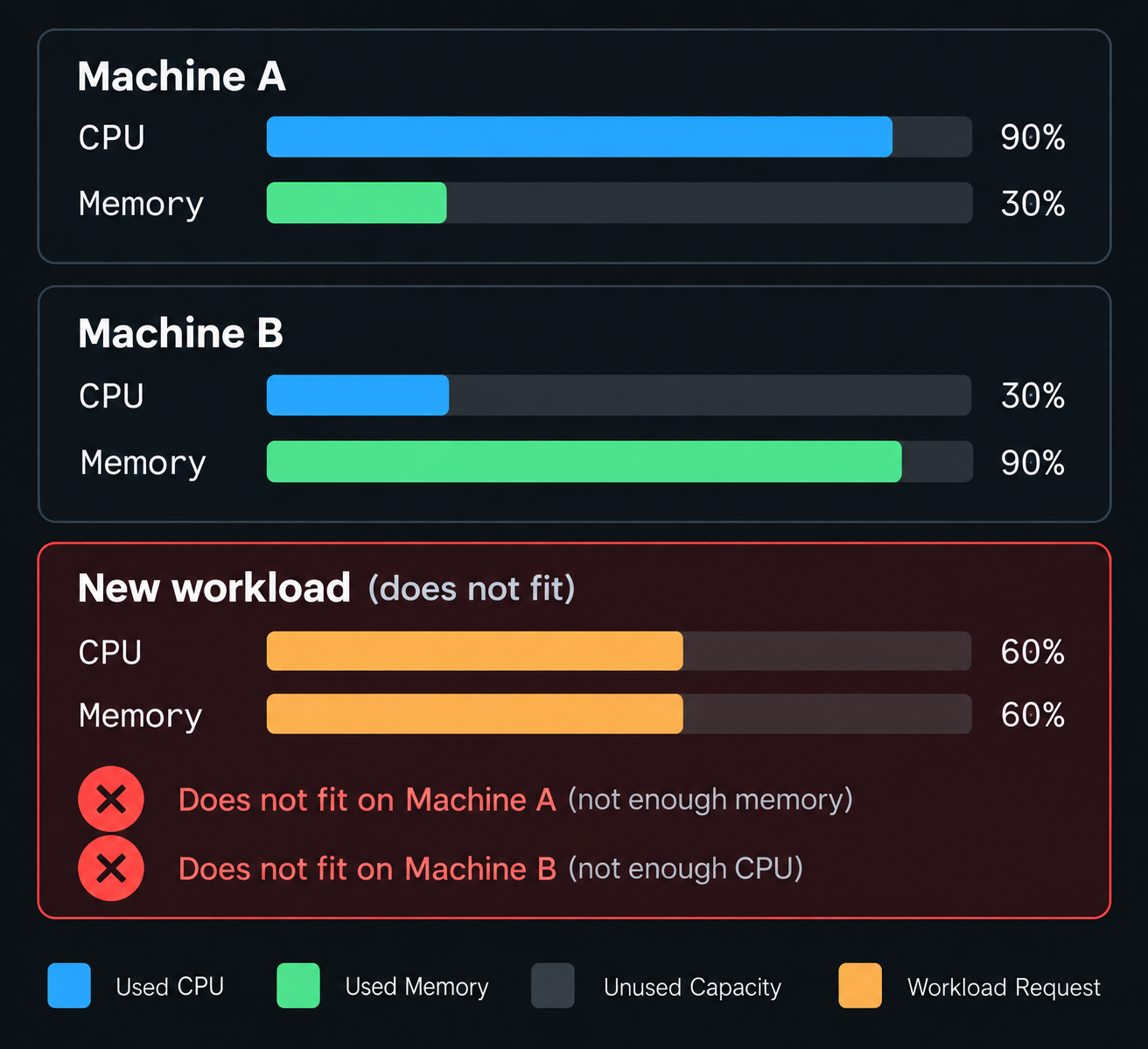
Neither machine has enough room for our new workload with balanced CPU and memory requirements. Yet if we look at the fleet as a whole, there's still plenty of unused CPU and memory:
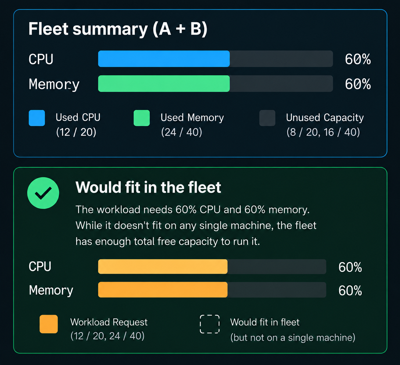
This means that our capacity is fragmented. It also means we have a lot of unused resources lying around. At scale, this situation leaves plenty of room for cost savings.
However real infrastructure is obviously more complicated than just CPU and memory. Depending on the workload, we may also care about storage capacity, IOPS and bandwidth, network throughput, local disks, GPUs or other accelerators, CPU architecture, topology, and various placement constraints.
This turns capacity optimization into a multidimensional bin-packing problem: given workloads with different resource requirements and machines with finite resources, how do we place those workloads so that we use the infrastructure efficiently while still leaving enough headroom for workload bursts and scaling, and without severely degrading performance? This is where things start getting interesting.
Bin-packing before Kubernetes
It's tempting to jump straight into Kubernetes here, because Kubernetes gives us a scheduler, resource requests and a very convenient vocabulary for this problem. But bin-packing existed long before Kubernetes, and I think it's useful to look at the simpler case first.
One common model is to use a dedicated VM for each service. But if a machine has spare CPU and memory, multiple workloads can share it. Containers make this much easier operationally, but the important primitive underneath is resource isolation. On Linux, cgroups let us put boundaries around CPU, memory and I/O usage so that packing workloads more tightly doesn't automatically mean letting them fight without limits.
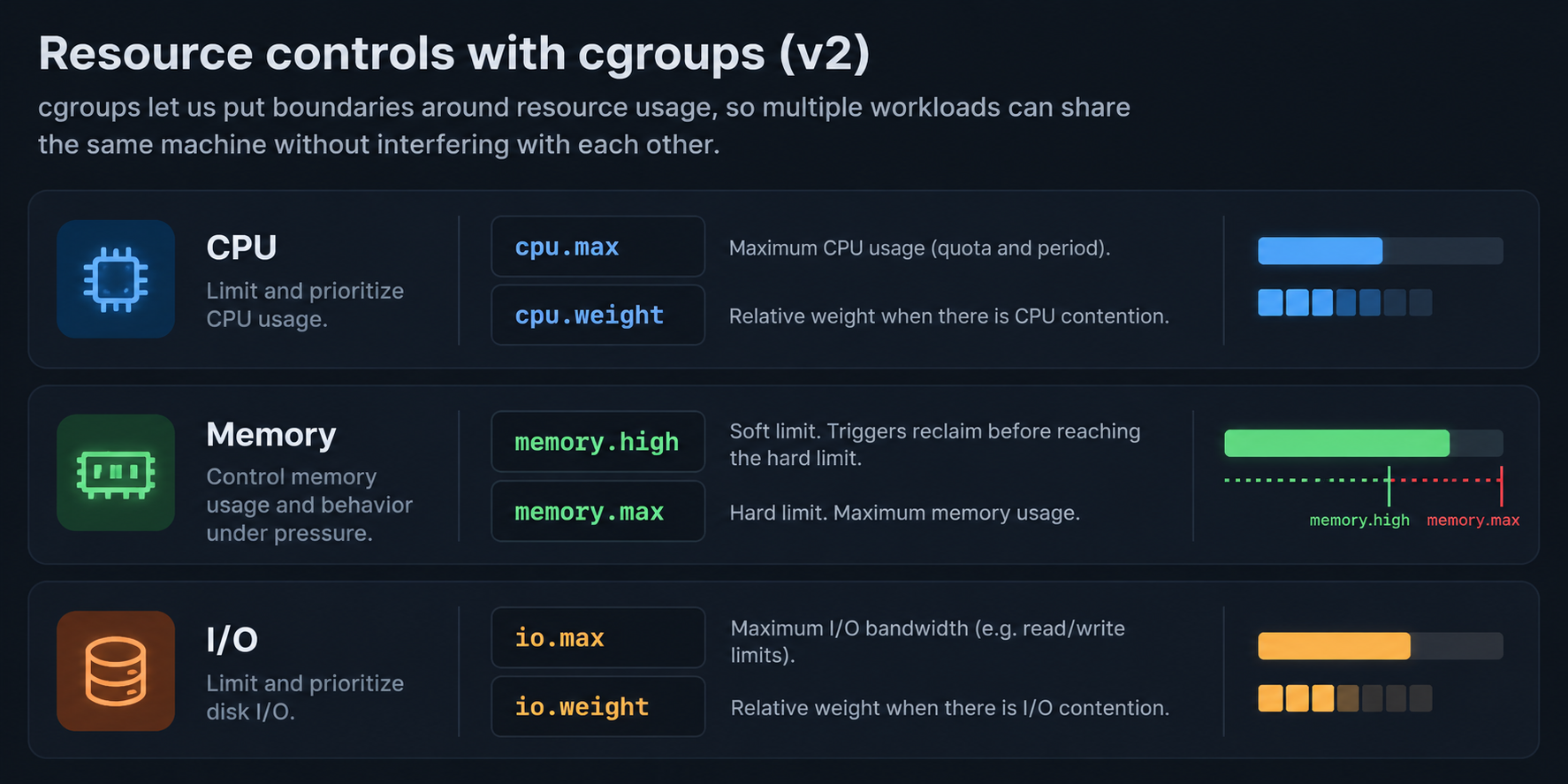
But let's not get into cgroups configuration here. The point is that efficient utilization requires two things at the same time: packing workloads together and maintaining enough isolation that one noisy neighbour doesn't destroy the performance of everything else on the machine.
Also, we need some headroom. How much depends on the workload, failure model and how quickly the platform can react. We may also need spare capacity for failover: if one machine disappears, the surviving machines must be able to absorb at least some of its work. So the target isn't 100% utilization. It's rather an experimentally determined threshold, and it can be a moving target. For instance: "generally we keep utilization around 80%, but in very constrained regions we're willing to push it closer to 90%."
How do we maintain such a level? Cgroups give us both resource controls and accounting. Apart from configuring limits and weights, the kernel exposes information such as CPU usage and throttling through cpu.stat, current memory consumption through memory.current, more detailed memory statistics through memory.stat, and I/O usage through io.stat. We can also observe resource pressure through PSI.
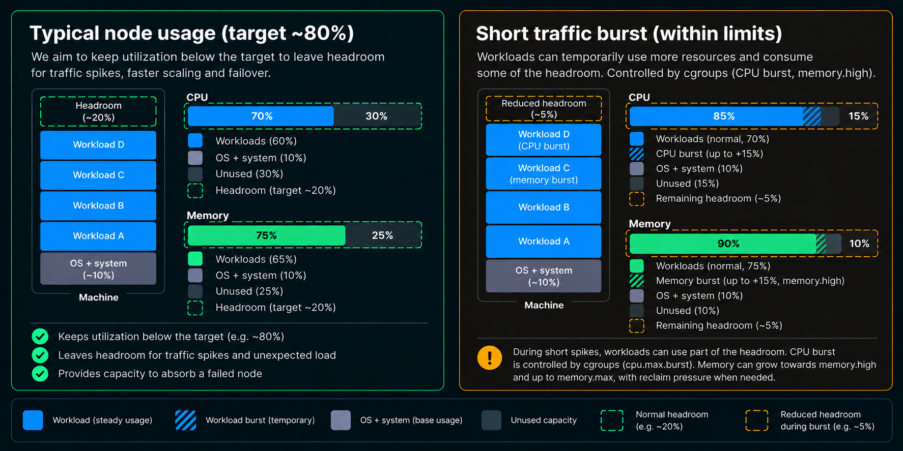
In the example above, the utilization target isn't necessarily a hard limit. If we aim for around 80%, the remaining capacity becomes headroom that workloads can temporarily consume during bursts, while still giving us some room for scaling and failures. Cgroups can help us control this behaviour - for example through CPU bandwidth and burst controls, or memory boundaries such as memory.high and memory.max.
Now we have both sides of the equation: controls that define how workloads may consume resources, and accounting that tells us what is actually happening on the machine. A custom application deployer or scheduler can use this information when deciding where to put the next workload. Let's say a new service needs 4 CPUs and 8 GB of memory. Instead of immediately provisioning another VM, our scheduler can first look at the existing fleet and ask: where can this workload fit without eating into the headroom we deliberately decided to keep?
But simply fitting isn't enough. Putting a CPU-heavy workload on a machine with plenty of CPU but almost no memory may be fine. Putting another memory-heavy workload there may not be. Likewise, choosing a VM where the new service consumes 50% of CPU while leaving 90% of memory unused might just create another badly fragmented machine.
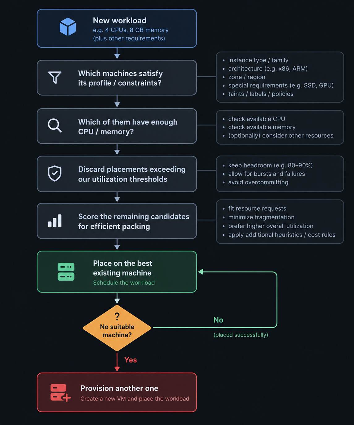
So there are several dimensions to the decision. First, the scheduler should narrow the candidates to machines compatible with the workload's infrastructure profile and other constraints. Then, among those candidates, it should prefer placement that increases utilization without crossing the configured safety thresholds and without unnecessarily fragmenting the remaining resources:
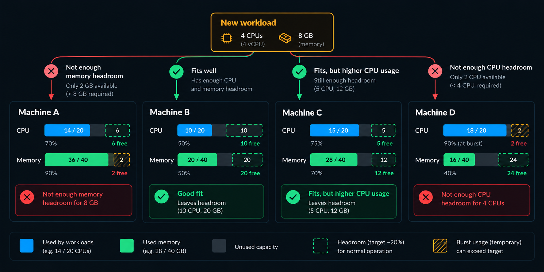
There is one caveat here. You probably noticed that this bin-packing problem can get very complex very quickly. The more variables we introduce, the larger the search space becomes. That's why it's a good idea to simplify it wherever we reasonably can. In the example above, we could intentionally limit our bin-packing decisions mostly to CPU and memory. Adding I/O - both storage and networking - introduces another world of complexity: disk performance, I/O schedulers, shared-device contention, network bandwidth, topology and so on. Cost-effective bin-packing is already complicated enough with CPU and memory alone. Conveniently, those are also the two main dimensions used to describe most general-purpose VM shapes and a significant part of what we're paying for.
That doesn't mean we shouldn't care about I/O performance - quite the opposite! I just wouldn't necessarily make every I/O characteristic another dimension of the bin-packing algorithm. Some of them may be better expressed as constraints or design requirements: "does this workload require local SSD?", "will those disks provide enough IOPS?", "what happens to network saturation when we reach 80% utilization?"
In other words, not every characteristic needs to become something we optimize. Some can simply tell us whether a particular placement is acceptable at all.
Conceptually, our scheduling decision could therefore look something like this:
And one last side note: we don't necessarily need a heavyweight container platform to get this kind of resource separation. systemd units can be placed into cgroups and configured with CPU, memory and I/O controls directly. If we need stronger process/filesystem isolation, systemd-nspawn is another relatively lightweight option.
I'm not arguing against Docker here - it's convenient, portable and makes developers' lives considerably easier. The point is simply that, at sufficient scale, it's worth remembering what's underneath all of this. Linux already provides the isolation primitives. Depending on what we're actually trying to achieve, using those primitives more directly can sometimes result in a simpler system.
And congratulations - we've just started building a scheduler 😄
Bin-packing within Kubernetes
For resource bin-packing specifically, kube-scheduler's NodeResourcesFit plugin supports strategies such as MostAllocated and RequestedToCapacityRatio. MostAllocated favors nodes that already have more resources allocated, while RequestedToCapacityRatio lets us shape the scoring function and weight different resources. That means CPU and memory don't even have to be treated equally - and extended resources can participate too.
This last bit can be quite useful. If the platform exposes something like local storage, accelerators or another scarce resource as an extended resource, it can participate in the scoring decision as well. This doesn't mean we should turn every possible characteristic into another optimization dimension - as discussed earlier, keeping the problem reasonably small is valuable. But when a third resource genuinely determines whether machines become stranded or useful, Kubernetes gives us a way to include it:
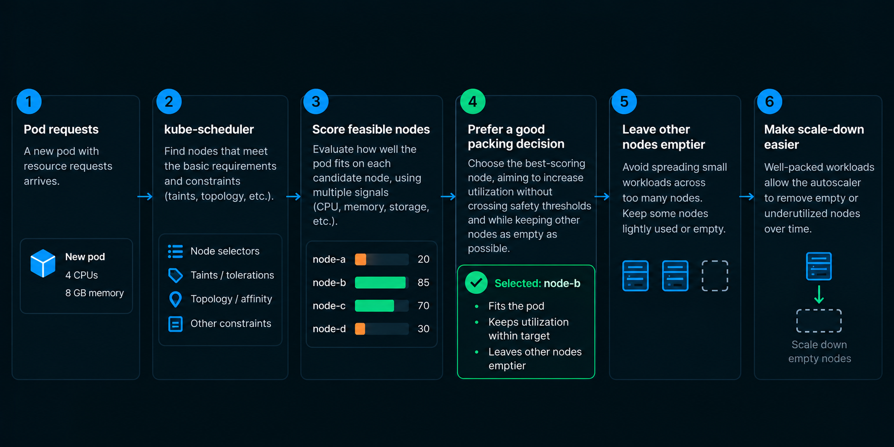
If workloads are distributed across a large fleet, we may end up with many half-empty nodes that are difficult to remove. Better placement can deliberately leave some nodes lightly used or empty enough that an autoscaler can eventually scale them down.
Of course, the scheduler is only as good as the information we give it. If requests are wildly oversized, the scheduler sees capacity that applications never actually use as already allocated. If requests are badly undersized, we may get excellent-looking packing right until contention starts. This is another reason why the rightsizing work from part 2 matters: application sizing and infrastructure utilization are two sides of the same problem.
There's another problem though: good scheduling doesn't guarantee that the cluster remains well packed over time. kube-scheduler makes a placement decision based on the state of the cluster at that particular moment. But that state changes continuously as workloads come and go, nodes get added or removed, and demand changes. Yesterday's perfectly reasonable placement may become today's fragmentation.
So besides making good initial placement decisions, we need some way to periodically reconsider the decisions we've already made.
This is where Descheduler comes in. It identifies Pods that should be evicted according to configured policies. For controller-managed workloads, once Pods are evicted, their controllers create replacements and kube-scheduler gets another chance to place them - hopefully somewhere better.
For our use case, HighNodeUtilization is particularly interesting. It identifies underutilized nodes and evicts suitable Pods from them so that those Pods can be compacted onto fewer, better-utilized nodes. The Kubernetes Descheduler project specifically describes this strategy as useful together with node autoscaling.
A simplified configuration could look something like:
pluginConfig:
  - name: DefaultEvictor
    args:
      nodeFit: true
      minPodAge: 8h

  - name: HighNodeUtilization
    args:
      numberOfNodes: 6
      thresholds:
        cpu: 60
        memory: 60

plugins:
  balance:
    enabled:
      - HighNodeUtilization
The 60% values aren't some universal recommendation - they're just an example. Here they tell Descheduler which nodes should be considered underutilized based on requested CPU and memory. In a real platform, those thresholds may differ between infrastructure profiles because different workloads have different performance characteristics and different amounts of safe headroom.
There are also several important guardrails in this example. numberOfNodes: 6 means we don't start moving workloads around just because we've found one lonely underutilized node. There needs to be enough potential consolidation to make the operation worthwhile.
minPodAge: 8h protects recently created Pods from eviction. This is important because a newly added node may naturally be underutilized for some time while the cluster is still converging. We don't want the Descheduler immediately fighting with scheduling and autoscaling decisions that have just been made. Notice that this is Pod age, not node age - it doesn't mean that a node must remain underutilized for eight hours.
Finally, nodeFit: true adds another safety check. Before evicting a Pod, Descheduler verifies that another node exists where that Pod could run, considering its resource requirements and scheduling constraints. Otherwise we'd risk evicting something only to discover that there's nowhere else to put it.
Put those together and the logic becomes roughly:
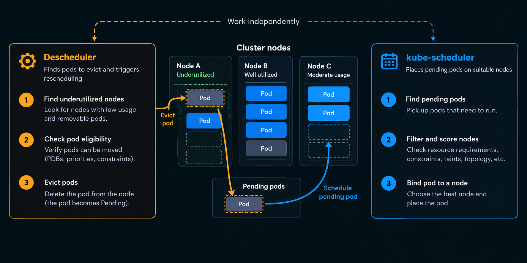
Time itself therefore becomes another dimension of our optimization problem. We don't necessarily want to react immediately just because the current state isn't optimal. Sometimes the correct thing to do is simply wait and see whether the condition persists.
This becomes even more important when several independent controllers are involved. We don't want an autoscaler to add a node, Descheduler to immediately reshuffle its newly scheduled workloads, and another controller to conclude that the node can now disappear again. In control-system terms, what we need here is hysteresis: deliberately requiring a meaningful enough change - or allowing enough time to pass - before acting again. In practice, this often takes the form of cooldown periods, minimum ages and persistence requirements.
We've actually already seen several examples. Descheduler's minPodAge can protect newly created Pods from immediate eviction, while its deschedulingInterval controls how frequently another descheduling cycle runs. Cluster Autoscaler has similar time-based guardrails: --scale-down-delay-after-add prevents scale-down evaluation immediately after adding capacity, while --scale-down-unneeded-time requires a node to remain unneeded for some time before it becomes eligible for removal.
None of these controllers needs to know exactly what the others are doing. They can operate independently, while these delays and thresholds give the overall system enough time to settle before another optimization decision is made.
Let's add Cluster Autoscaler to the picture. Its job is different; Descheduler can help empty an underutilized node, but it doesn't terminate that node. Cluster Autoscaler can identify that the node is no longer needed, check whether its remaining Pods could be moved elsewhere, and eventually remove it. For example, we might configure something along these lines:
--scale-down-utilization-threshold=0.75
--scale-down-delay-after-add=10m
--scale-down-unneeded-time=60m
--balance-similar-node-groups=true
--expander=priority,least-waste
A scale-down-utilization-threshold of 0.75 means we're willing to consider relatively well-utilized nodes as potential scale-down candidates, so that's quite an aggressive setting compared with the current default of 0.5. Cluster Autoscaler calculates this using Pod CPU and memory requests, not actual CPU and memory consumption.
Notice the two time-related settings as well. scale-down-delay-after-add prevents Cluster Autoscaler from immediately reconsidering scale-down after adding capacity (hysteresis!), while scale-down-unneeded-time requires a node to remain unneeded (an internal Cluster Autoscaler classification, not a Kubernetes Node state) continuously for some time before it becomes eligible for removal (hysteresis again!).
balance-similar-node-groups becomes useful when we have equivalent node groups - for example similar capacity spread across availability zones - and want Cluster Autoscaler to keep their scale-up reasonably balanced. It applies to scale-up, though; it doesn't mean CA maintains identical group sizes during scale-down.
And expanders are interesting in the context of the infrastructure profiles from part 2. Cluster Autoscaler needs to decide which node group to expand when several of them could satisfy pending Pods. With:
--expander=priority,least-wastewe can first express our preference between node groups, and then use least-waste to choose among remaining candidates based on the CPU and memory that would be left unused after scaling.
Put all three components together and we get a nice feedback system, which includes many independent reconciliation loops:
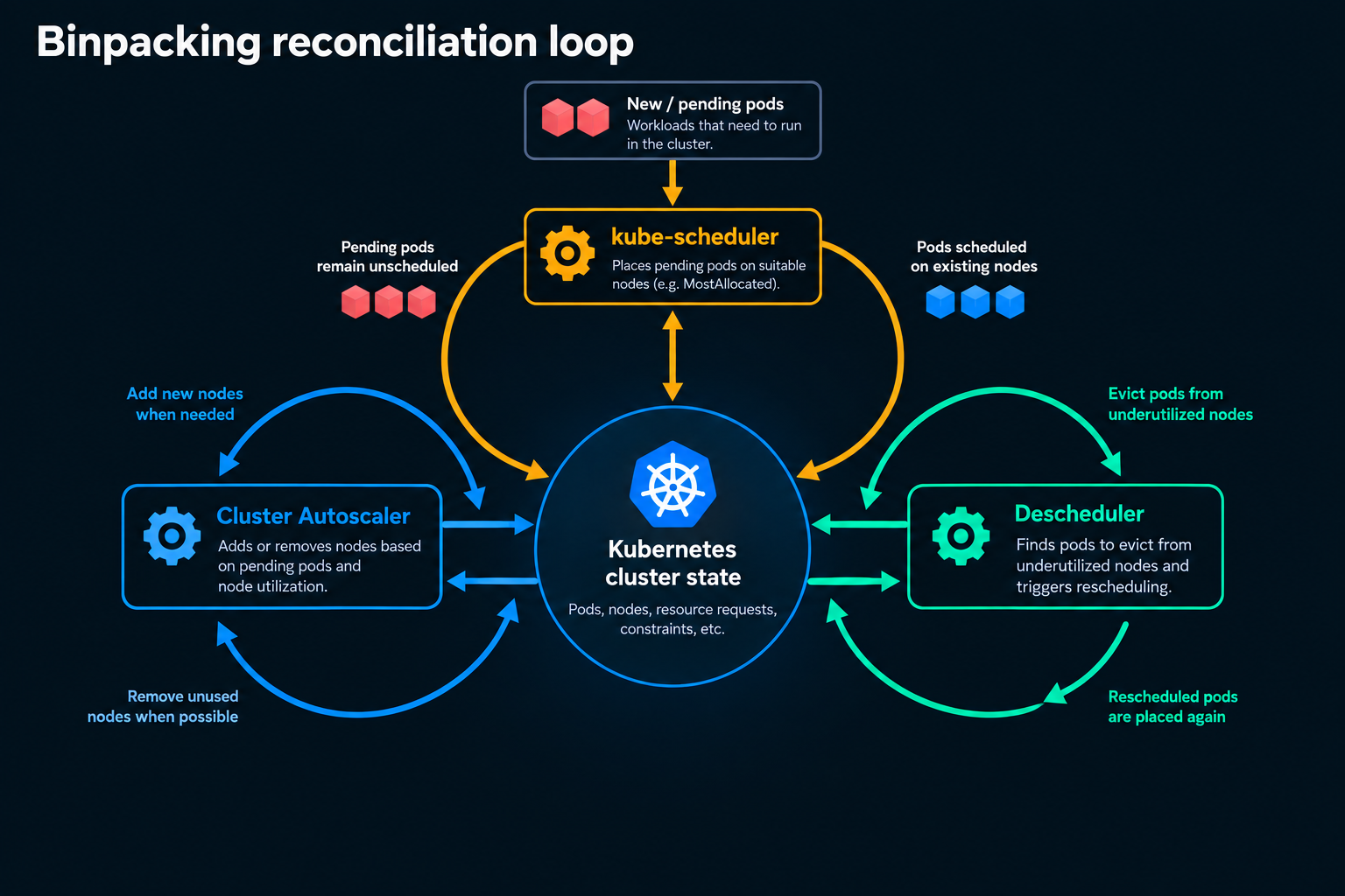
Put together, this is really what bin-packing is about. We're not trying to achieve the highest possible utilization just because a graph looks nicer at 80% than at 50%. We're trying to run the required workloads reliably on less infrastructure, while deliberately keeping enough headroom for bursts, failures and scaling.
Better utilization therefore eventually translates into something much less abstract: fewer machines and a lower infrastructure bill.
What's next?
But there's an assumption underneath everything we've discussed in this part: the capacity already exists. Which brings us back to where this series started: forecasting capacity is useful, but eventually we need to secure that capacity, manage it and continuously reconcile what we need with what is actually available. And once we try doing that across many projects, regions, infrastructure profiles, quotas and reservations... things get interesting again 😄
That's where Part 4 starts. And yes, that's also where we'll finally get to:
Forget Terraform. Just code it. Well... sort of. 😄


Comments